Static perfect hashing in minimal memory

Sometimes we want to build a static dictionary data structure. This is when we have a set of data that doesn’t have to change dynamically. When it changes, we can just rebuild the dictionary from scratch. So we first build the data structure, and then perform lookups without changing it any more.

Example scenarios where we might want to do this:

• Spell checker. We have a set of words that doesn’t change, and want to perform lookups to see if a word is spelled correctly.
• Search engine. We periodically crawl a lot of web pages and build an index containing all the words, with links to the pages. Once the index is built, we don’t change it, until we do a new crawl again

What we want is:

1. Linear build time in expectation. So for $n$ elements of size $S$ words each, we want to be able to build the data structure in $O(nS)$ expected time. If elements are of constant size, this is $O(n)$ time.
2. Guaranteed quick access time to all elements. We want $O(S)$ time per access. If the element size is constant, this is $O(1)$ time.
3. Not much memory overhead. We are aiming for memory use of $nS + o(n)$. Note that $nS$ is just the space required to store the elements. So this means that for large $n$ the fraction of extra memory required for bookkeeping is small compared to the actual data.

As usual, we are using the “word RAM” computational model. What we mean by a “word” is a piece of memory that can store a pointer or a number in the range of 0 to $n$. So a word has at least $\log n$ bits. Note that if we have $n$ distinct elements to store in the hash table, they necessarily have at least $\log n$ bits each, or else they couldn’t be distinct.

For a while it was an open problem whether such a data structure (or even just properties 1 and 2) is even possible. In 1984 Fredman, Komlós, Szemerédi¹ described a data structure that does this.

One could try to just use a regular hash table with universal hashing. It sort of works, but it fails properties 2 and 3. We get constant access time, but only in expectation. No matter how many hash functions we try, there will almost surely be some buckets that have more than a few entries in them. In fact it can be shown that if we use a completely random hash function to store $n$ elements in $n$ buckets, then with high probability the largest bucket will have $\Theta(\log n / \log \log n)$ entries. For universal hashing it could be a lot worse. A few customers could get angry that their queries are always slow! We don’t want that. We would also have significant memory overhead to store all the buckets and pointers.

Guaranteeing worst case access time

Start by defining a family of universal hash functions such that the probability of a collision when hashing into $m$ buckets is bounded by $c/m$ for some constant $c$. Normally we can make $c \approx 1$.

Now let’s create $n$ buckets and randomly select a hash function $H$ that maps elements to those buckets. The expected number of collisions, i.e. the number of pairs of data elements that hash to the same bucket, is bounded by:

$$\sum_{0 \le i < j < n} \Pr(H(x_i) = H(x_j)) \le \binom{n}{2} \frac{c}{n} < \frac{n^2}{2} \frac{c}{n} = \frac{cn}{2}$$

The probability that the number of collisions exceeds twice the expectation, i.e. $cn$, is at most 50% (otherwise the expected value would be larger). If that happens, we just try again and pick a different $H$. It will take on average 2 tries to get a valid $H$.

Thus we have at most $cn$ collisions.

Let $b_i$ be the number of elements in bucket $i$. Then the number of collisions can also be expressed as:

$$\sum_{i=0}^{n-1} \binom{b_i}{2} \le cn$$

Now comes the main trick: in each bucket let’s make another, second-level mini hash table!

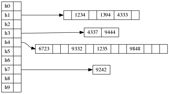
We size a given secondary table based on its number of elements. Make it $\max\left(2c\binom{b_i}{2}, 1\right) = \max(cb_i(b_i-1), 1)$ (note that this is quadratic in the number of elements). Select a random hash function $h_i$. We want no collisions in the second level hash table.

The expected number of collisions in a given second level hash table is bounded by:

$$\binom{b_i}{2} \frac{c}{\max\left(2c\binom{b_i}{2},1\right)} \le \frac{1}{2}$$

So with probability at least 50% we don’t get any collision at all! In case we get a collision, just try a different $h_i$. After an average of 2 attempts we will get zero collisions in that table.

So we don’t need any secondary collision resolution method. Just store pointers to elements directly in mini-buckets.

A lookup is now constant time:

1. Calculate $i = H(x)$
2. Calculate $j = h_i(x)$
3. The element, if it exists, will be in bucket $i$, entry $j$.

Total space used for second level hash tables is:

$$\sum_{i=0}^{n-1} \max\left(2c\binom{b_i}{2}, 1\right) \le 2c\sum_{i=0}^{n-1}\binom{b_i}{2} + n \le 2c \cdot cn + n = (2c^2+1)n = O(n)$$

Memory overhead is therefore $\Theta(n)$. It is not negligible, especially if the actual data elements are small.

Compression

Now we are aiming to reduce the memory overhead to $o(n)$, i.e. something that is relatively small for large n.

First, let’s increase the number of main buckets by a factor of $z$ (to be determined later), so we have $zn$ buckets. Seems like this will only make it worse, but bear with me. We will pack them really tightly!

The expected number of collisions is now smaller:

$$\sum_{i=0}^{zn-1} \binom{b_i}{2} \le \binom{n}{2} \frac {c}{zn} < \frac{n^2}{2} \frac{c}{zn} = \frac{cn}{2z}$$

Again, we make sure that we don’t get more than twice that, i.e. $cn/z$. If we do, just try a different hash function $H$.

If $b_i = 1$, we are not going to have a second level hash table. Instead, we will store a pointer to the element directly in the main bucket.

For $b_i \ge 2$, we make a second level hash table of size $2c\binom{b_i}{2} = cb_i(b_i-1)$. This again means that we can easily get zero collisions in each such table.

The total size of all second level hash tables (and thus also the number of such tables) is bounded by:

$$\sum_{i=0}^{zn-1} 2c\binom{b_i}{2} < 2c \frac{cn}{z} = 2c^2 \frac{n}{z} = O\left(\frac{n}{z}\right)$$

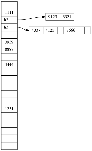
Now let’s put all the data elements into a dedicated array. Order them so that the ones that appear in single-element buckets are ordered first, in the same order as they appear in the buckets. Also put all the secondary table hash functions and pointers into a separate array, again in the same order as they appear in main buckets. In the main bucket table we just need to store what kind of entry it is (none, single element, or secondary table), and an index into the appropriate array.

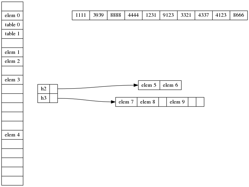
Finally, we group the main buckets into groups of size $g$. In each group we store just one index of the first single element in the group (if any), and one index of the first secondary table in the group (if any). In each individual bucket we just store an offset from those. The above bucket table now looks like this:

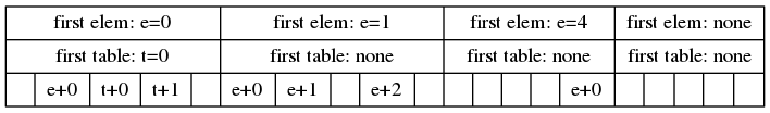
There are $zn/g$ groups. In each group, we need 2 words for the first element index and the first table index, for a total of $2zn/g$ words.

We also have $zn$ individual buckets. Each bucket has the type of bucket (there are 3 types, so 2 bits), and an offset. However, those offsets are small, between 0 and $g$. So buckets only need $2 + \log g$ bits each. We can pack them into $O(zn \log g / \log n)$ words, because we know we can fit $\log n$ bits in a word.

The total space usage for all the elements, all the secondary tables, and all the buckets is therefore:

$$nS + O\left(\frac{n}{z} + \frac{zn}{g} + \frac{zn\log g}{\log n}\right)$$

Now we’ll pick $g$ and $z$ to make this as small as possible. Start with the group size $g$. We want the last two terms to be approximately equal, which means $g\log g \approx \log n$, or $g=\Theta(\log n / \log \log n)$.

This makes the memory usage:

$$nS + O\left(\frac{n}{z} + \frac{zn\log \log n}{\log n}\right)$$

Finally optimize the number of buckets $zn$. Again we want the two terms to be approximately equal, or $z = \Theta(\sqrt{\log n / \log \log n})$.

The final memory usage then is:

$$nS + O\left(n \sqrt{\frac{\log \log n}{\log n}}\right) = nS + o(n)$$

Asymptotically smaller than linear overhead! Just as we wanted.

References

1. Fredman, Michael L., János Komlós, and Endre Szemerédi. “Storing a sparse table with O(1) worst case access time.” Journal of the ACM (JACM) 31.3 (1984): 538-544. ↩