Tournament-winning gomoku AI

• Introduction
• Rules
• Example game 1
• Threats
  • Five
  • Open four
  • Simple four
  • Open three
  • Broken three
  • Non-forcing threats
• Example game 2
• Precomputed patterns
• Static evaluation
• Board representation
  • Rotated bitboards
  • Threat Boards
  • Incremental static evaluation
• Threat sequence search
  • All-defenses trick
  • Dependency-based search
  • Counter-threats and refutations
• Principal variation search
  • Defenses to potential threat sequences
  • Null move forward prunning
  • Panic mode
• Opening book
• Conclusion
• References

Introduction

I’m going to describe my Gomoku playing program that I submitted for CodeCup 2020. The program (named “OOOOO”) ended up winning the tournament, placing first in a field of 58 entries, and winning 98 out of 100 games.

CodeCup is an excellent annual tournament for game AIs organized by the Dutch National Olympiad in Informatics. Every year they host a tournament for programs playing a game, with a different board game each time.

In January 2020 the game was Gomoku. It was a bit unusual in that the game chosen was a well-known game. Usually it’s a completely new game, or an obscure game not well known. So I thought that winning submissions might be some existing programs that were already developed previously over many years. This turned out not to be the case.

I enjoyed coding this game very much. The game has very simple rules, and allows very interesting algorithmic ideas.

You can see the results and all the games on the tournament website.

Rules

The game was simple “free-style” gomoku played on a 16x16 board. Players alternate placing black and white stones anywhere on the board, until somebody makes 5 stones in row horizontally, vertically or diagonally, which wins.

To minimize first-player advantage, “swap rule” is employed. One player makes the first three moves (black, white, black), and the other player may choose to continue with white, or swap colors.

Example game 1

Take a look at an example game played between OOOOO (black) and Leopold Tschanter’s “ltgmk” (white).

The game ended with the following sequence:

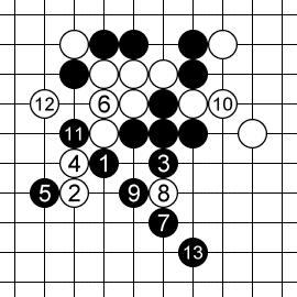
When OOOOO played the move marked as 1, it already knew it was going to win, 13 ply (7 moves) before the game ended. This despite the fact that the space of possible moves is very large: each player has almost all 256 intersections available each move.

The endgame is a forcing sequence of threats to which defenses are more or less forced.

Move 1 is a diagonal “simple four” threat. 2 is forced, otherwise black will play at 2 and win immediately.

Move 3 is a diagonal “broken three” threat.

This time however, white doesn’t have to respond immediately. Instead, he makes a stronger counter-threat with a simple four at 4. Black has to defend the counter-threat at 5.

Now white has to go back and address the threat at 3. If he ignored the threat, black would make a diagonal “open four” threat at 6 to which there would be no defense.

So white defends at 6.

Now black makes another simple four at 7. White has to respond at 8.

Now black makes a double “open three” threat at 9. White doesn’t have a good counter-threat, so defends one of these open threes at 10.

Black converts the other, undefended open three into an open four with 11. There is no defense to an open four (other than making an immediate five). White defends on one side with 12, and black finishes with a five on the other side at 13, winning the game.

Pretty much every gomoku game ends in one of these long forcing threat sequences. It is therefore essential to be able to find such sequences and defend against opponent’s sequences.

Threats

We categorize threats as follows:

• Winning threats. There are fives and open fours.
• Forcing threats, i.e. opponent must respond. These are: simple fours, open threes, and broken threes.
• Non-forcing threats. These don’t require the opponent to respond, but may become forcing threats later when additional stones are added.

Winning and forcing threats can also be ordered by their severity:

• Fives.
• Fours.
• Threes.

This ordering will useful when thinking about counter-threats later. Instead of answering a forcing threat, one may counter with a more severe forcing counter-threat.

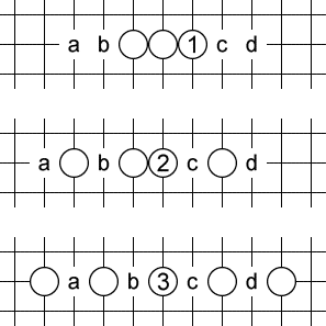
Five

Fives are pretty self-explanatory. You immediately make five in a row and win. 1, 2, 3 are fives.

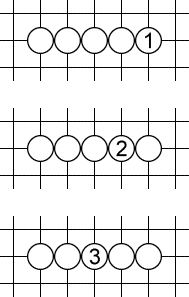
Open four

A standard open four threat is a play like 1. Black has no defense. If black plays at a, white plays at b. If black plays at b, white plays at a. The only way to salvage the game for black would be to play a more severe counter-threat elsewhere, i.e. a five!

But 1 is not he only pattern like that. 2 and 3 work exactly the same way. They also create two ways for white to finish the game. Even though they involve 6 and 7 stones rather than 4, I also call such equivalent patterns “open fours” (because we have four stones out of five in a row).

Simple four

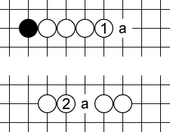
A simple four is a forcing threat, threatening a five next move, but only in one way. It doesn’t necessarily win, but forces a response. White plays at 1 or 2, black has to respond at a (or play a more severe threat, i.e. a five).

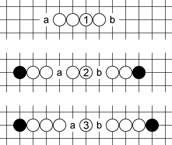
Open three

The most common open three looks like 1: three in a row, with at least two empty spaces on each side. Black has to defend at b or c (or play a four-threat elsewhere). Otherwise, white will make an open four at b or c and win.

Open three is a special kind of threat in that four empty spaces are required, but only two of them are valid defenses for black. For instance, if black tries to defend at a, white still makes an open four at c and wins. This will be relevant later, when we talk about sequences of threats: we have to make sure that a and d are still empty when this threat is played, even though black can’t defend there.

And again, there are other patterns like 2 and 3 above that we call “open threes” even though they involve more than three white stones. The defining characteristic is that there are four empty spaces of which white needs to fill any two consecutive ones to win.

The last pattern (3) is my favorite. It looks pretty. And it played a major role in example game 2 shown below.

Broken three

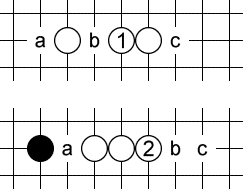
Finally we come to the weakest type of forcing threat, but probably the most common one: a broken three. Here only three empty spots are involved. Black can defend at any one of them, otherwise white will make an open four at b.

Non-forcing threats

All types of threats can be described by two numbers: $(a,b)$ where $1 \le a \le 5$ is the threat severity (we already have $a$ stones out of 5), and $1 \le b \le 6-a$ is the number of possible ways to make a five.

So all the threats types are as follows:

• Winning threats:
  • (5, 1): five
  • (4, 2): open four
• Forcing threats:
  • (4, 1): simple four
  • (3, 3): open three
  • (3, 2): broken three
• Non-forcing threats:
  • (3, 1): simple three
  • (2, 4), (2, 3), (2, 2), (2, 1): a two that can be extended to a five in 4, 3, 2, 1 ways respectively
  • (1, 5), (1, 5), (1, 3), (1, 2), (1, 1): a single stone that can be extended in 5, 4, 3, 2, 1 ways respectively
• No threat at all

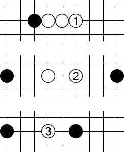
All the above are non-forcing threats. Play at 1 is (3, 1), i.e. a simple three. Play at 2 is a (2, 3), a two that can be completed in 3 ways. Play at 3 is not a threat at all, because it can’t make five in a row in this direction.

Example game 2

Let’s look at another game from the tournament. OOOOO plays black versus Sjoerd Hemminga’s SjoerdsGomokuPlayer playing white.

The final forcing sequence that OOOOO employed looks like this:

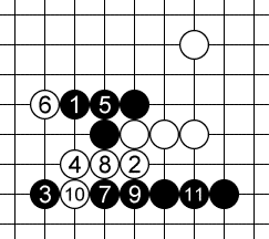
Black plays a diagonal broken three at 1, white defends at 2. Black plays another diagonal broken three at 3, white defends at 4. Black plays a horizontal open three at 5, black defends at 6.

And now comes a pretty double-threat at 7. A standard vertical broken three, and a nice non-standard horizontal “open three” consisting of four stones, all separated by empty spaces.

White defends the vertical threat at 8, and black converts the undefended horizontal “open three” into a non-standard “open four” (actually consisting of five stones) with 9. White defends one of the two spots at 10, and black finishes the job at 11.

Precomputed patterns

My bot has a lot of things precomputed, to enable a quick recognition of threat patterns.

There are 16 types of threats (from no threat to a five). There are a total of 65 distinct threat patterns. For each pattern we store the set of squares that must be occupied, the set of squares that must be empty, and the set of squares that are possible defenses.

For each line length from 5 to 16, and for each pattern of opponent stones on that line, we precompute how the line is split into sub-lines by opponent stones. Any threat has to be contained within a sub-line.

For each sub-line length from 5 to 16, and for each pattern of our stones, we precompute what threat patterns are available within the subline.

Using these tables we can quickly look up threats available on the board for each player.

Static evaluation

My static evaluation of a position is very simple. I tried some simple machine learning, but ended up just using a simple hand-made formula that works reasonably well.

For each player, and for each empty intersection of the board, I look at what threats are available for that player at this intersection in the four direction. I take two best threats, and assign them numbers from 0 (no threat) to 16 (immediate five) based on the threat type.

If the two best threats at intersection i have values $a_i$ and $b_i$, my evaluation for one side is:

$$\sum_{i\in\text{empty}} (1.5 \cdot 1.8^{a_i} + 1.8^{b_i})$$

Total static evaluation is the difference of single-side evaluations, plus a bonus for the side to move.

Board representation

We want the board representation to be a data structure that supports some important operations efficiently:

• See if the game is over and who won.
• Make a move.
• Un-make a move (to support recursive game tree search).
• Compute the static evaluation.
• Find all winning or forcing threats for each player (to start the search for a winning threat sequence).

Our board representation consists of:

• Rotated bitboards.
• Threat Boards.
• Incremental static evaluation.

Rotated bitboards

A bitboard is a sequence of 16x16 = 256 bits. We could represent the board as two bitboards: one for black stones and one for white stones.

We add redundancy so that we can easily extract patterns of bits corresponding to lines on the board. For each player we store the board in four copies, rotated by 0, 90, 45 and 135 degrees. So we have:

• A row-major bitboard, where intersections in the same row are consecutive.
• A column-major bitboard, where intersections in the same column are consecutive.
• A NW-SE bitboard, where intersections in the same NW-SE diagonal are consecutive.
• A NE-SW bitboard, where intersections in the same NE-SW diagonal are consecutive.

Threat Boards

For each player we maintain a Threat Board. A Threat Board contains information about each square in each direction. For empty intersections, we store the current threat pattern available in that square.

Every time we make or un-make a move, we update all threats in the neighborhood. We look up the pattern in each direction in our precomputed tables, and update all threats nearby. We have to go a distance of 4 in each direction, so we only have to update 8 * 4 = 32 nearby intersections.

We also keep track of whether the game is already over, so we can answer that question immediately.

Incremental static evaluation

Every time the current threat available at an intersection is updated, we recompute the score for that intersection, and update the total sum of these scores. This way we have the score always available without having to recompute it for the whole board.

Threat sequence search

This is the central and most compute-intensive part of the whole program. Every time we encounter a new position, we want to be able to tell whether there exists a winning combination of threats for the player to move. We also want to be able to tell whether there exists a winning combination of threats for the other player, and if so, how the current player can defend against it. In the tree search we will only consider those moves that defend against such combinations.

The algorithm for finding these threat sequences is inspired by the Ph.D. thesis of Victor Allis, “Searching for solutions in games and artificial intelligence.”¹

All-defenses trick

Consider a threat sequence like this:

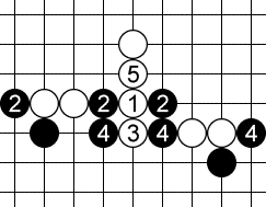
White first plays a horizontal broken three at 1. Black can defend it at any of the three points marked as 2. Now white plays another horizontal broken three at 3, and again black can defend it at any of the three points marked as 4. Finally, white plays a vertical open four at 5 and wins the game next move.

If we were to search the game tree in a straighforward way, there are 9 different combinations here, because black can defend the first threat 3 ways, and the second threat 3 ways. But all of them are very similar, it’s essentially the same sequence.

We avoid checking all these combinations separately by using the trick discovered by Victor Allis. When searching for a winning threat sequence for white, we simply assume that black is allowed to play all the defenses to a single threat at once!

This is a conservative approach, but often good enough, and saves a lot of computation.

So above we simply say: first we play the first threat, which adds a white stone at 1 and three black stones at 2, 2, 2. Then we play the second threat, which adds a white stone at 3 and three black stones at 4, 4, 4. Then we play the final game-winning threat at 5.

This trick avoids some of the combinatorial explosion of the number of cases, and makes the threat search a single-player game.

Dependency-based search

Another way to reduce the number of combinations to look through is to notice that in the combination above, the order of the first two threats doesn’t matter. We could play 1 first, or we could play 3 first. We don’t need to check both orders separately. For longer sequences, this helps a lot.

This algorithm is again due to Victor Allis’ Ph.D. thesis¹.

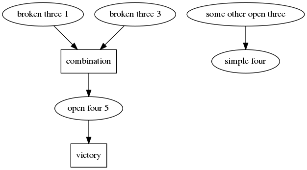
Instead of searching for sequences of threats, we search the dependency graph of threats.

In the example above, threat 5 depends on threats 1 and 3.

We start from all immediate threats. For each threat node, we look at whether new threats are enabled by this threat, and create those nodes.

We also combine threats that are on a single line (such as 1 and 3) into “combination nodes”, and look for new threats that are created as a result of such a combination.

Before we create a combination node we check whether the two threats that we are combining, and their dependencies, do not interfere with each other (i.e. reuse the same squares).

When combining threats, special care is taken for open threes. An open three allows only two defense points, but requires two additional intersections to be empty when the threat is executed. These empty intersections can later be used for other threats. This creates additional ordering dependencies between open threes and other threats. When combining threats, we use topological sorting to see whether we can order threats so that these ordering dependencies are satisfied.

We thus build a directed acyclic graph of threat nodes and combination nodes, until we run out of possibilities, or we find a game-winning threat (open four or five).

Counter-threats and refutations

If only things could be that simple…

Imagine we have found the following threat sequence:

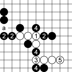
White plays a horizontal broken three at 1 (it’s not an open three due to the presence of a black stone), then a vertical broken three at 3, then a horizonal open four at 5, which wins.

It looks good. But it doesn’t work. Black can use the left-most 2 as a defense to 1. Then, after white plays the threat at 3, black ignores the threat, and instead plays a more severe counter-threat at a creating an open four and winning the game!

This is a refutation of a threat sequence. While playing out his own threats, white inadvertently helps black set up counter-threats that ultimately defeat the threat sequence.

There are two ways a threat sequence can be refuted by counter-threats:

• The defender may win with his own counter-threats.
• The defender may use his counter-threats to place a stone at a spot where it interferes with the original threat sequence.

After finding a threat sequence with the dependency-based search, we run another dependency-based search, this time for defender’s counter-threats, to see if we can find a refutation. Differences from regular search are:

• We look at counter-threats after each move of the original threat sequence. These may combine with counter-threats made in response to other, earlier threats in the threat sequence.
• We only consider counter-threats that are more severe than the original threat.
• We declare victory for the defender when either he wins or manages to interfere with the original threat sequence.
• We don’t consider refutations to refutations recursively. Instead, if we find a potential refutation, we just conservatively assume that it works, throwing away the potential threat sequence that we found.

Principal variation search

As the main game tree search algorithm, we use Principal Variation Search, which is a variant of alpha-beta prunning. In each node we run dependency-based search to see if a threat sequence is available, and also whether the current player has to defend against opponent’s possible threat sequence.

Defenses to potential threat sequences

In each node of the tree search, we run dependency-based search for the opponent of the player to move, to see if there is a potential danger we have to defend against.

If there is, we first want to determine the set of moves that defend against the danger.

We augment the dependency-based search algorithm to also return all moves that could potentially be defensive moves, whenever a winning sequence is found. These potential defensive moves are:

• all intersections that are part of the threat sequence, and
• all intersections that create additional counter-threats for the defender in the refutation search

Once we have this set of potential defenses, we try each one in turn, and again run the threat search for the other player.

• If the threat search now returns no attack for the opponent, we have found a valid defense, so we add it to the set of valid defenses.
• If it does return another winning threat sequence, then this potential defense doesn’t work. But also we then get another set of potentially valid defenses to this other threat sequence. A defense that works has to work against all threat sequences, so we take the intersection of the two sets of potential defenses.

We continue this until we have converged on the set of defensive moves that work. This set could be empty, which means that the position is lost, and we can score the node in the tree.

If it is not empty, we only consider those moves that are valid defenses as children of the tree node.

Null move forward prunning

Some moves don’t create any potential winning threats. Often these are weak moves. We want to try to prune these from the search tree.

The way this is implemented is similar to the null-move heuristic often used in chess programs.

If in a node there is no threat sequence for the opponent, there is no immediate danger. In that case, we first try a null move, i.e. no move at all, and run a shallower search. If this shallow search returns a good score (a beta-cut in the alpha-beta algorithm), we assume that this position is really good for the player to move. It probably is, since he doesn’t even have to move to get a good score. So, in that case, we never search this subtree to a full depth and just score the node as a good score.

Panic mode

Suppose we completed our search to depth N, and found a drawish score. Then we start a depth-(N+1) search, and consider the currently best move. It turns out that the move loses! Oops! So we start trying other moves. But at this point we run out of allocated time for the move. What to do?

We enter panic mode.

In panic mode, we ignore whatever time we had allocated for this move, and continue searching other moves. We continue looking until we have found a move that doesn’t lose, or we have tried every possible move and they all lose, or we have really run out of all most of the time on the clock.

Opening book

We only use an opening book when we are playing black. The black player chooses the opening, i.e. the first three moves. I picked that opening manually, trying to put the moves in the center of the board to create a nice fight, and to make chances for the two players as equal as possible, according to my bot’s evaluation (that’s what we want because of the swap rule).

Using a simple algorithm by Lincke², I automatically constructed an opening book for my chosen opening. The book contains 1379 positions that were analyzed off-line by the program.

Conclusion

This was a fun coding exercise!

Potential ideas I had that I didn’t have time to try:

• Better static evaluation, using machine learning.
• Proof number search instead of alpha-beta pruning. Proof number search is probably well suited for gomoku, because it is a very tactical game. It would allow searching some tactical lines much deeper than others. Interestingly, this algorithm was also designed by Victor Allis in the same Ph.D. thesis!¹
• Instead of one evaluation function, use two evaluation functions, showing potential for each player separately. Some positions are very “offensive” (which would be a high score for both players) and some are “defensive”, locked-down (low score for both players). When looking for a win for one side (as in proof number search), one player should prioritize offensive positions, and the other player should try to defuse the situation by reducing the offensive potential of the opponent.

Maybe I’ll try these in the future if there is another Gomoku AI tournament.

References

1. Allis, Louis Victor. Searching for solutions in games and artificial intelligence. Wageningen: Ponsen & Looijen, 1994. ↩ ↩² ↩³

2. Lincke, Thomas R. “Strategies for the automatic construction of opening books.” International Conference on Computers and Games. Springer, Berlin, Heidelberg, 2000. ↩